3D velocity model with complex geology and voids for microseismic location and mechanism


3D velocity model with complex geology and void
for microseismic location and mechanism
Deep Mining 2014 – M Hudyma and Y Potvin (eds)© 2014 Australian Centre for Geomechanics, Perth, ISBN 978-0-9870937-9-0
DS Collins ESG Solutions, Canada
Y Toya ESG Solutions, Canada
I Pinnock ESG Solutions, Canada
V Shumila ESG Solutions, CanadaZ Hosseini ESG Solutions, Canada
Abstract
A microseismic monitoring system provides a vital window into a rock mass to see where stress induced fracturing is occurring in relation to mining operations. A main factor for the accuracy of the microseismic locations is the velocity model assumed for the rock mass. The majority of mines that use microseismic systems use a single velocity model for location purposes which assumes the same elastic modulus properties throughout the volume. This study shows examples of event locations that were calculated using a velocity model that accounts for multiple complex shaped geological units each with their own properties. The method allows multiple voids to be added that could be air filled, brine filled, or cement paste back filled, thus mimicking mining and geotechnical operations such as stope mining, cave mining, solution mining, or underground cavern storage.Going beyond the dots, microseismic systems provide an important way to understand the failure mechanics of the rock fracturing. With good data quality, each located event can be solved for the source mechanism (moment tensor) and interpreted in terms of whether the event is dominantly tensile opening, closing, or shear slip. The orientation of each event failed zone can be quantified providing useful information about the discrete fracture network (DFN). This paper provides examples of source mechanism solutions using a full 3D velocity model. It is shown that the ray path of each sensor does affect the source mechanism solution when comparing a single velocity model solution and a 3D velocity model solution.Microseismic systems offer important daily information for mine operation, safety and planning. Improvements to the accuracy of seismic results by using enhanced processing methods and regular calibration, allow a mine to more confidently integrate seismic results with numerical models and make decisions. This is especially important as mines move to different excavation methods such as block caving and extend to greater depths and stresses.
1. Introduction
Many mining applications around the world are using microseismic monitoring as an essential tool to listen to the way a rock mass is responding to stress changes and provide immediate notice of abnormal behaviour such as large magnitude events or clusters of events (Alexander & Trifu 2005; Hudyma et al. 2010; Wu et al. 2012). Forensic seismic analysis within a few days of abnormal activity or even months later can provide an important assessment of the source parameter trends, as well as the mechanics of failure in respect to mine excavations and faults (Trifu et al. 2007; Collins et al. 2013, 2014). This can help mines make a more informed decision for mine design and safety.Recently, microseismics are playing an essential role in applications such as the monitoring of shale gas hydraulic fracturing and underground storage caverns (Baig et al. 2012). Being able to monitor a 3D volume of rock deep under the ground in real time is very important for tracking any rock fracturing and coalescence that may be occurring.
2. Microseismic monitoring
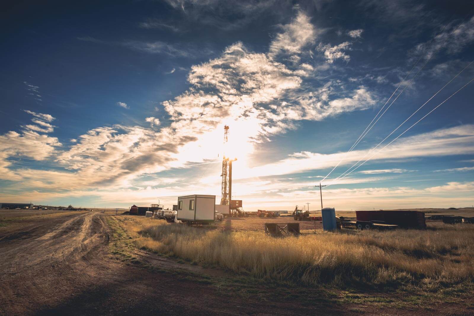
Microseismic systems in mines have changed considerably over the past 25 years. Modern systems can digitise over 100 events per minute and provide a seismic alert of abnormal activity within one minute of it occurring. The systems are modular with sensors and digitising units placed underground for high signal to noise quality. Continuous digitised data with GPS time synchronisation is passed over a fibre optic network to a surface computer where it is saved to a large ringbuffer hard drive, along with the triggered event data. The ringbuffer drive allows mine operators to go back a number of weeks and investigate seismic events using a more sensitive trigger setting in areas of interest. Figure 1 is a schematic drawing of an example mine being monitored with surface and underground sensors. Trained operators in the engineering office are able to use 3D visualisation software to depict the mine and seismic results to make informed decisions about mine operation and safety.
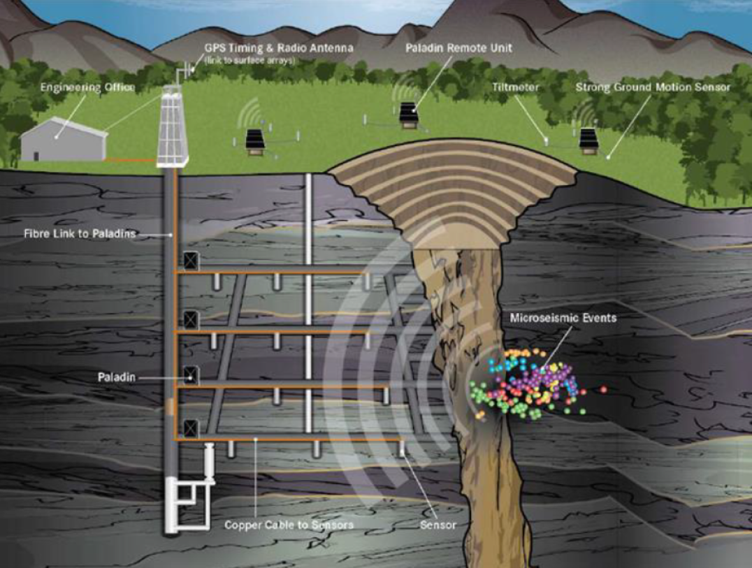
Fig. 1. Example of a typical microseismic system setup. Energy from microseismic events is recorded on sensors installed underground and above ground. The networked data is received at a central engineering office for real time processing and results display
Many hard rock mines have a sensor array that allows them to record microseismic events down to moment magnitude (MW) of -3 (source dimension about 1 m). Piezoelectric accelerometer type sensors are generally needed to record to this small magnitude size. Fifteen Hz geophone type sensors can record microseismic events down to about MW = -2.0. For weak or soft rock mines, it is recommended to use 15 Hz geophones since the energy from events MW<-2.0 will be strongly attenuated, making the use of accelerometers not ideal unless they are very closely spaced. 4.5 Hz geophone type sensors, also known as strong ground motion (SGM), are generally used to record events MW>0.0. Figure 2 is a schematic figure showing the recommended magnitude range for the three sensor types discussed. A combination of theSeismicityDeep Mining 2014, Sudbury, Canada 683three sensor types can result in the magnitude range -3.0<MW<3.0 being covered in specific regions of the rock mass. SGM sensors can detect and locate events with MW>3.0, but will generally slightly underestimate the true magnitude. Lower frequency range sensors, such as a 1 Hz geophone, can be used to complement a sensor array if very large magnitude events are expected.
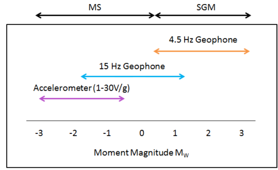
Fig. 2. Graph showing the recommended magnitude range for accurate source parameter calculation from different sensor types. A mixture of the three sensor types shown can allow a system to be sensitive to a six order of magnitude range. The lower frequency sensor is termed SGM while the other two sensor types are termed microseismic (MS)
A 3D distribution of sensors is an ideal configuration and will generally lead to the highest accuracy in source locations and parameters. A 2D (planar) or 1D (linear) distribution of sensors can also be used as a microseismic array and provide good quality results. 2D sensor arrays are commonly used in certain mine types such as coal mines and salt mines. In the case of 2D or 1D sensor arrays, it is important to have some triaxial sensors installed to avoid non-uniqueness in the location solution. Figure 3 shows how two possible locations, identified as 1 and 2 above and below the plane, can occur when using a subplanar array of uniaxial sensors. The use of a mixed array of uniaxial and triaxial sensors will lead to a unique solution (identified as location 3). This is because triaxial sensors can provide P-wave arrival time and direction information compared to uniaxial sensors which just provide arrival times.
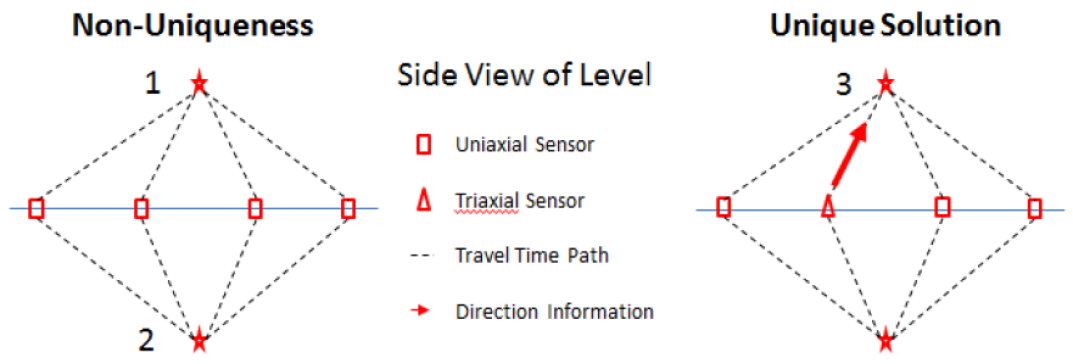
Fig. 3. Schematic showing the importance of both uniaxial and triaxial sensors in a planar underground array. Two possible location solutions (stars identified as 1 and 2) exist when locating with uniaxial sensors. The addition of a triaxial sensor strategically into the array identifies the correct location (star identified as 3)
3. Rock mass velocity model
The accuracy of seismic locations and source parameters are significantly affected by the velocity model (VM) assigned to the rock mass. A simple assumption is to use a single VM (e.g. isotropic, homogeneous) and use known location sources (e.g. blasts or significant impacts) to determine the best single velocity value and quantify the absolute location accuracy. A more complex VM type involves multiple parallel layers with or without anisotropy. The most complex VM type is one that allows multiple 3D shapes and voids. This paper builds on work by Trifu and Shumila (2010) and Collins et al. (2014) that develop location algorithms which can use 3D VMs that account for complex geological shapes and voids. Collins et al. (2014) show an 87% improvement in location accuracy when accounting for mine stopes in seismic location at a hard rock mine.
3.1 Seismic locations from case study one
Case study one is an underground cavern in North America that is being monitored by a mixture of uniaxial and triaxial microseismic sensors installed in four vertical boreholes (Figure 4). Using sonic log surveys from the four boreholes, six main layers were identified. A 3D VM was developed that used the six horizontal layers as well as the 3D shape of the cavern. Data from surface drop tests recorded on the sensors was used to optimise velocity values for each of the six layers. The brine filled cavern was assigned a P-wave velocity of 1,615 m/s (5,300 ft/s).Figure 5 shows a north–south cutting plane through one of the sensor boreholes and cavern. Time isolines (isochrons) are shown from the dot based on the 3D VM being used in the analysis. As expected, the isolines are seen to vary when passing between the horizontal layer boundaries and also as a result of the low velocity cavern zone. The star shows an example seismic event location. The black curved line connecting the star to the dot is the expected path for the fastest seismic energy to take. It is seen to go around the cavern instead of through part of the cavern if a more simple (straight ray path assumption) VM had been used.
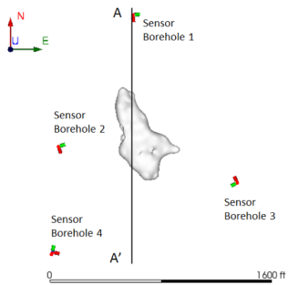
Fig. 4. Plan view of case study one showing the underground cavern (grey surface) and microseismic sensors. Line A-A’ identifies a vertical section shown in Figure 5
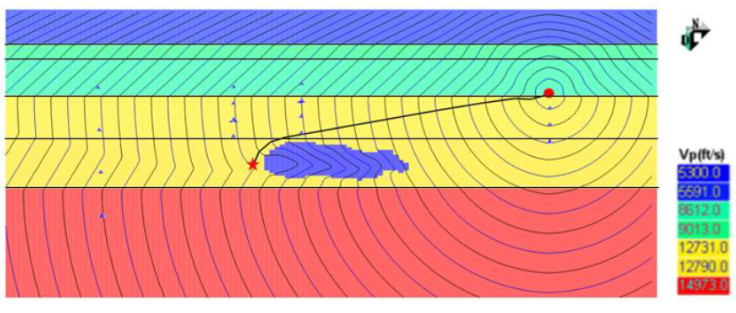
Fig. 5. The 3D VM consists of six horizontal layers (the six main geological units) and the brine filled cavern. The image shows time isolines from the dot (time zero). Significant changes in the isolines are noticed at layer boundaries and inside and around the cavern. The curved black line shows the direct (fastest) path for seismic energy from the dot to the star location.
3.2 Seismic locations from case study two
Case study two is a block cave mine in a moderate strength rock mass in North America. The 3D VM that was developed comprises of five irregular 3D shaped geological units with subvertical boundaries. Additionally the block cave volume was incorporated as an air filled void. Figure 6 is an image of a seismic event (filled circle) located using the 3D VM. A mixture of uniaxial and triaxial microseismic sensors is shown as black symbols and the cave void is displayed. The curved lines from the event to each sensor show the fast seismic energy path using the 3D VM. As expected, ray bending occurs at geological unit boundaries as well as significant ray bending around the void. At regular stages of cave growth, the 3D VM is updated.
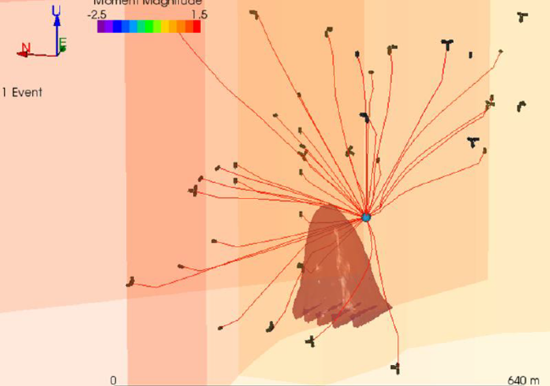
Fig. 6. A seismic event (filled circle) locating near an underground cave void. The seismic sensors are the black symbols. The lines are the direct (fastest) paths for seismic energy from the event to the sensors accounting for the cave void and five geological units at the site. Significant ray bending is noticed around the cave void
3.3 Seismic mechanisms from case study two
Seismic mechanism analysis in mines generally involves the calculation of the moment tensor (MT) with no a priori assumption about the mechanism type (Trifu & Shumila 2002; Collins et al. 2002). This allows all types of failure to be possible such as shear slip, tensile opening, or crack closure. The method used here is seismic moment tensor inversion (SMTI) and it has been developed to use a 3D VM. SMTI requires the seismic energy direction to each sensor, and also a distance correction to each sensor amplitude. The use of a calibrated 3D VM will provide more accurate input information (energy direction and amplitude) than a simpler VM.Figure 7 shows the MT solution for an event in case study two inverted using a single VM and 3D VM. The results are shown on a lower hemisphere stereonet projection with the centre representing vertical from the source and the sides of the hemisphere representing horizontal orientations from the seismic source. It is noticed that the data points (filled circles) vary by up to 10° in location on the hemisphere between the single VM and 3D VM. This is due to the differences in the energy paths between the event and sensors for the different velocity models. This difference will affect the final mechanism solution. In Figure 7(a), straight ray paths are assumed, and in Figure 7(b) variable ray paths can occur around voices and through different geological units. More significant variations can occur when seismic events locate very close to underground caverns or voids.
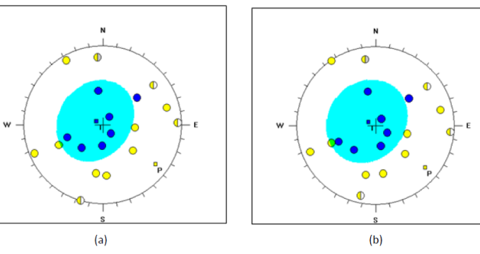
Fig. 7. Source mechanism (moment tensor) solutions for the same event calculated using (a) a single velocity model; and (b) a 3D velocity model. The filled circles represent sensor data points with positive (dark fill) and negative (light fill) P-wave first motion, respectively. The results are presented on a lower hemisphere stereonet projection. Data point locations are different by up to 10° when comparing (a) and (b)
In Figure 8, a group of 20 microseismic events are displayed from case study two. In (a) the events are shown as equal sized dots in relation to the cave void (object below events). In (b) the events are shown with their SMTI mechanism solutions in a beach ball representation. For each event the dark regions signify outwards strain and the white regions inwards strain. The majority of the highest elevation events have a dominant shear slip mechanism while the lower elevation events have a dominant opening type mechanism. In (c) each event is displayed as a 3D strain tensor with outwards strain shown as away facing dipole arrows and inwards strain shown as in facing dipole arrows. There is a noticeable trend of subhorizontal inwards strain and subvertical outwards strain.Based on Trifu and Shumila (2011), a stress tensor was determined from the cluster of source mechanism results. This seismic stress tensor method can use any type of source mechanism and was developed for mining applications. It is an enhancement of the method of Gephart and Forsyth (1984) which was developed for earthquake studies and assumes shear slip failure. In Figure 8(d), the mechanism results are shown as circular fractures scaled to their calculated source radius. For event mechanisms that are dominantly shear slip (greater than 50% shear in MT), the stress tensor determined for the cluster has been used to resolve which of the two possible shear slip planes are more likely to have slipped. For the remaining events, the fracture plane displayed is assumed to be perpendicular to the opening or closure direction (largest inwards or outwards strain). The group of fractures shown is considered a DFN. The display of source mechanism results as a DFN offers additional information about the fracturing occurring in the rock mass relative to mine voids, and is helping seismic interpretation to go beyond the dots.
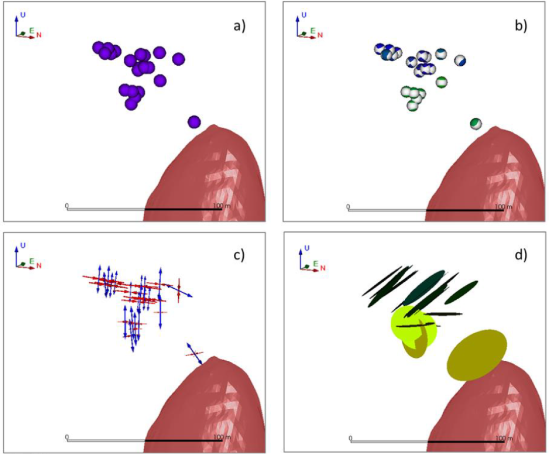
Fig. 8. Seismic events occurring near to a void (large shaded surface in bottom right) in case study two. In (a), the events are shown as dots found using a 3D VM. In (b), the source mechanism solutions are shown as a beach ball type display. In (c), the source mechanism solutions are shown as a strain tensor, and in (d) the solutions are shown as discrete fractures sized to their source dimension. See text for further details
4. Conclusion
This paper presents results from two case studies in North America. In case study one, the use of a 3D VM with six horizontal layers and the 3D shape of the brine filled cavern is allowing microseismic events to be more accurately resolved, especially those occurring near to the boundaries of the cavern. In case study two, a 3D VM was developed that accounts for five irregular shaped 3D geological units as well as a cave void, and was used to determine source locations and mechanisms of a group of 20 events. As expected, the use of a 3D VM is shown to affect the source mechanism solution compared to the use of a single VM. Source mechanism results are displayed in three different ways (beach balls, strain tensor, and DFN), with the latter involving the use of seismic stress tensor inversion. It is hoped that the use of source mechanism analysis can become more commonly used in seismic analysis to help understand the mechanics of failure associated with the rock fracture locations.
References
Alexander, J, Trifu, CI 2005, ‘Monitoring mine seismicity in Canada’, in Y Potvin and M Hudyma (eds), Proceedings of the Sixth International Symposium on Rockburst and Seismicity in Mines: RaSiM6, Australian Centre for Geomechanics, Perth, pp. 353-358.
Baig, A, Urbancic, T & Wuesterfeld, A 2012, ‘Variability of hydraulic fractures in shale or tight gas reservoirs’, in RF Broadhead (ed.). Proceedings of the Tenth Middle East Geosciences.
Conference, American Association of Petroleum Geologists, Tulsa, Article #90141.
Collins, DS, Pettitt, WS & Young, RP 2002, ‘High resolution mechanics of a microearthquake sequence’, Pure Applied Geophysics, vol. 159, pp. 197-219.
Collins, DS, Pinnock, I, Toya, Y, Shumila, V & Trifu, CI 2014, ‘Seismic event location and source mechanism accounting for complex block geology and voids’, in P Smeallie & J Roberts (eds), Proceedings of the 48th ARMA US Rock Mechanics/Geomechanics Symposium, American Rock Mechanics Association, Alexandria, paper 14-7530.
Collins, DS, Pinnock, I, Shumila, V, Trifu, CI, Kamp, C, Davies, A & Chan, A 2013, ‘Optimizing microseismic source event location by applying a variable velocity model to a complex geological and mining setting at the New Gold New Afton Block Cave’, in FP Hassani (ed.), Proceedings of the 23rd World Mining Congress on Advances in Mining Engineering, Canadian Institute of Mining, Metallurgy and Petroleum, Westmount, PDF paper 674.
Gephart, JW & Forsyth, DW 1984, ‘An improved method for determining the regional stress tensor using earthquake focal mechanism data: application to the San Fernando earthquake sequence’, Journal of Geophysical Research, vol. 89, pp. 9305-9320.
Hudyma, MR, Frenette, P & Leslie, I 2010, ‘Monitoring open stope caving at Goldex Mine’, Proceedings of the Second International Symposium on Block and Sublevel Caving, Australian Centre for Geomechanics, Perth, pp. 133-144.
Trifu, CI & Shumila, V 2002, ‘The use of uniaxial recordings in moment tensor inversions for induced seismic sources’, Tectonophysics, vol. 356, pp. 171-180.
Trifu, CI & Shumila, V 2011, ‘The analysis of stress tensor determined from seismic moment tensor solutions at Goldex Mine Quebec’, in P Smeallie & J Roberts (eds), Proceedings of the 45th ARMA US Rock Mechanics Symposium, American Rock Mechanics Association, Alexandria, paper 11-584.
Trifu, CI & Shumila, V 2010, ‘Geometrical and inhomogeneous raypath effects on the characterization of open pit seismicity’, in P Smeallie & J Roberts (eds), Proceedings of the 44th ARMA US Rock Mechanics Symposium, American Rock Mechanics Association, Alexandria, paper 10-406.
Trifu, CI, Shumila, V & Burgio, N 2007, ‘Characterization of the caving front at Ridgeway Mine, New South Wales, based on geomechanical data and detailed microseismic analysis’, in Y Potvin, J Hadjigeorgiou & TR Stacey (eds), in Challenges in Deep and High Stress Mining, Australian Centre for Geomechanics, Perth, pp. 445-453.
Wu, X, Liu, C, Hosseini, Z & Trifu, CI 2012, ‘Applications of microseismic monitoring in Chinas underground coal mines’, in TM Barczak (ed.), Proceedings of the 31st International Conference on Ground Control in Mining, pp. 130-137, Published by International Conference on Ground Control in Mining, West Virginia.