

By Trevor K. C. Pugh
Introduction
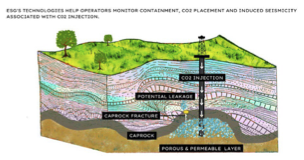
Carbon capture, usage, and storage (CCUS) has become an essential technology to aid in the reduction of greenhouse gas emissions. The greatest concern regarding CCUS is
the environmental risk associated with long-term storage of captured CO2. Any containment breach and leakage would likely negate the initial environmental benefits of capturing and storing CO2 emissions.
This technology was labeled for many years as low risk technology due to the low rates of injection. The most common monitoring methods for CCUS largely focus on monitoring the risk of containment breach and caprock and/or well integrity. This is generally thought of as capacity limitations and permanence of containment at a storage facility. Several studies have highlighted the risk of induced seismicity due to the injection of CO2.
ESG Solutions has collaborated with an operator to provide long-term seismicity monitoring for a project in Alberta, Canada. The operator’s team utilizes the collected microseismic data to update the site's geo-mechanical model. The study has also demonstrated the importance of continuous monitoring during injection operations to ensure storage control and containment permanence.
In addition, it was noted that the types of data recorded and methods of collection will vary over time in order to provide a consistent and cost-effective solution.
From ESG’s experience, the main monitoring objectives for CCUS operations are:
- Risk reduction
- Containment
- Fault activation avoidance
- Induced Seismicity
- CO2 Plume extent
- Caprock integrity
We know from geomechanical modeling that the pressure caused by CO2 injection should not create new fractures or activation of existing faults due to the low rates of the injection and capacity of the reservoir. Therefore, altering the stress regime during the CO2 injection job has been the subject of several studies and linked as the main factor of triggering microseismic events.
It was evident during the long-term monitoring of this project that the lateral extent and integrity of the caprock was not a factor of any direct measurement with microseismic monitoring.
However, there are electromagnetic imaging technologies utilized over the past 15 years that are proving useful in monitoring deep fluid injection for hydraulic fracturing, flowback detection, and EOR analysis. This paper will discuss the implementation of electromagnetic imaging combined with microseismic analysis for monitoring in the CCUS space.
Recent developments in the understanding of Controlled Source Electromagnetic (CSEM)monitoring for fluid injection have provided an important supplemental tool for monitoring long-term containment of sequestered CO2.
Background
CO2 injection commenced in 2015 at the Quest Carbon Capture and Storage (CCS) Facility located near Fort Saskatchewan, Alberta, Canada. The CO2 is injected into a deep saline aquifer at a depth of 2km. Minimal seismicity was expected with these CO2 injections but as noted in Figure 2 below, the long-term increases in built up stress caused a growth in recorded seismicity over time.
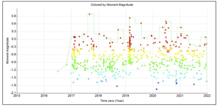
The data strongly suggests that long term-monitoring for potential effects from CCUS operations is largely important. However, knowledge of the capacity and long-term stability of the project will be enhanced by understanding the full extent of the plume migration and caprock integrity. This is where electromagnetic imaging can be of great assistance to CCUS operators.
CSEM Scattered Field Responses and how they work
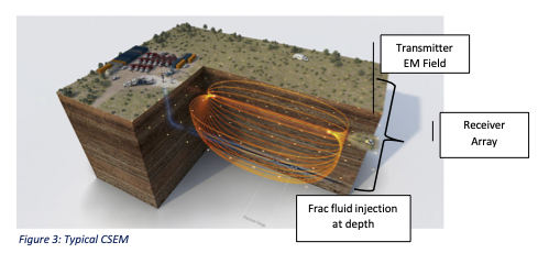
For those unfamiliar with onshore CSEM technology being used at ESG Solutions, please see references [8,9,10]. A typical onshore CSEM design, shown in Figure 3, has the following components:
- A surface-based array of electric field sensors, sensitive in the nano Volt region
- A surface array of receivers and transmitters that are precisely timed to within 10's of nano seconds with no drift over time
- A surface-based transmitter that can produce significant power (250KW is currently available)
- A surface-based transmitter that uses a pseuro-random numeric (PRN) code to produce a designed broadband, flat, low frequency signal that is stable over man days and has the same frequency content as near infinite impulse.
- This is currently a 2D X, Y map - vertical fluid fill can be implied with signal strength and rock damage by phase changes over time
- A time-lapse difference field or scattered field response is recored and displayed.
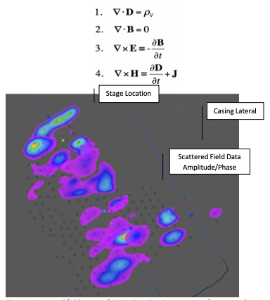
To create a 2D image of fluid injection, the total electric field measured at the start of the fluid injection operation subtracted in the frequency domain from the readings as injection continues. This produces a scattered field response in both amplitude and phase.
The scattered field response is directly correlated to the subsurface fluid activity, as can be seen in Figure 4 showing field data.
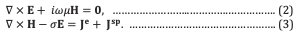
Typically, in the CSEM world, these responses have been modeled using well-understood forward modeling methods based on solving Maxwell’s equations (quasi-static) shown below. These methods are applicable to large stationary resistive/conductive targets that are the targets of offshore exploration. However, as will be explained in this paper, fluid injection modifies the physical mechanisms which are not adequately described in those equations because they can be treated as additional ‘transmitting’ sources to generate EM fields.
Streaming Potential (SP)
The conventional Streaming Potential (SP) method is a passive geophysical tool which measures naturally occurring electric fields or voltages created by fluid flow through geologic formations [4,5]. The widely recognized applications of SP techniques range from monitoring dam leakage, estimating the hydraulic conductivity in hydrogeology, monitoring volcano and geothermal activities, and well logging in the oil and gas industry [1,3,6,7]. One advantage of the SP method lies in its ease of data acquisition, without an actively man-made exciting source.
Combining this response with an active CSEM source on the surface allows for the detection of both SP and EM responses. The interesting factor here is that SP responses occur at much higher frequencies than would be expected in an arrangement without a CSEM transmitter. This leads to a unique measuring system that is responsive to the following signals in combination:
- Streaming Potential caused by pressure and flow rate changes
- Conventional CSEM resistivity measurements
- Advanced CSEM responses that include frequency-based changes in impedance, reactance, and reluctance (resistance, mutual inductance, and capacitance)
Dielectric Constant at low frequency in rock
In addition, there has been significant work done by the Colorado School of Mines [12]relating to the low frequency dielectric constant for various rock types from cores. The work shows that not only must the dielectric constant (permittivity ratio) be fully considered in EM modeling at low frequencies, but that it is a large value (10^6) and anisotropic by up to a factor of 100:1.
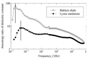
This leads to a new understanding of the phase response from CSEM data. The phase change is strongly correlated with rock damage. Cracking a layered rock changes the vertical dielectric constant causing a detectable change in phase. For more details on this subject see reference [11].
Discussion and Data Examples for Streaming Potential and CSEM
As shown in Figure 6, in this CSEM data, the measured electric scattered fields (bottom panel) at one sensor located at the surface and close to the injection well in a shallow operation, show strong correlations with the injection well borehole pressure (blue) and pump flow rate (red). This suggests dominance of the SP signal in the measured CSEM data.
However, one of the unexplained issues with this observation is the frequency content in the measured EM data. The EM trace along time in Figure 6 are the scattered responses at100 Hz, while commonly accepted SP signal should be close to DC.
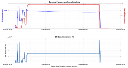
An inconsistency is noted between the observed CSEM scattered field data and the conventional SP signal in terms of the frequency content.
Additionally, the signal strength of the CSEM scattered field as predicted by the usual 3D EM modeling at low frequencies is approximately 1 to 2 orders of magnitude smaller than observed. This is a further inconsistency between observed and expected data.
The following figures show other real-world examples of this relationship:
Figure 7 depicts an additional example from a hydraulic fracturing operation where the relationship between pressure, injected fluid, proppant, and the transmitter normalized scattered field CSEM response for a frac at ~3000m of depth at 10Hz.
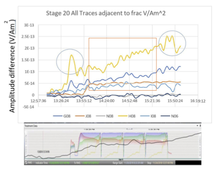
There are many features within Figure 7 that should be noted:
- Response delay for the sensors that are further away in horizontal distance from the frac location
- Suggestion of more than one signal type, as is typified by the blue circles and the red box
- Large response at the onset of pumping
- Smaller responses taking longer to be expressed in the data – typical for CSEM
- Data heavily localized to the surface array that is vertically adjacent to the frac stage
All of these features in the data and some additional unpublished data from the University of Texas Devine test site, provide impetus for a revision of EM equations relating to fluid flow and CSEM combined as it is discussed below.
Modeling comparison with field data
Figure 8 below demonstrates that modeling including both 3D EM and SP can resolve the difference between the signal collected in the field and signal predicted by analytic SP solution and 3D EM modeling.
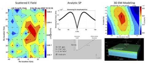
Note that the 3D EM modeling on the right-hand side predicts a maximum voltage of~3.5e^-7V/m and the actual data on the left is measured at 5e^-6 V/m. The addition of the SP modeling in the center image resolves this discrepancy to a greater degree. A full matching of the observed data leads to the following spCSEM method.
A New spCSEM Modeling Algorithm (patent pending)
Based upon the understanding of the mechanism of SP under an external EM exciting source, a new spCSEM modeling algorithm is proposed here. Besides the normal exciting current 𝐉𝐞, the streaming potential current 𝐉𝐬p can be treated as an additional source for generating the spCSEM’s electromagnetic signal. The streaming current 𝐉𝐬p� can be obtained by equation (1)

where L is the cross-coupling coefficient between a fluid and electric flow in the coupled flow theory [1,2,5], and p is the pressure field, which may be solved in a reservoir simulation or geo-mechanical platform. Therefore, the modified frequency-domain EM equations for spCSEM might look like:
Then by solving these equations, both electric and magnetic fields can be computed. This constitutes the spCSEM frequency-domain forward modeling engine, which can be used in the following inverse problem. From the spCSEM inversion, the conductivity or conductivity change of the injected fluid can be inferred.
Extending the spCSEM method for application in CCUS
Firstly, it is worth noting that ESG Solutions has provided CSEM data to clients for hydraulic fracturing, flow back, and EOR operations. Flowback operations have flow rates per foot(meter) of the well and pressure regimes that are of the order of those that would be expected within CCUS. In addition, ESG Solutions has extensive experience in passive microseismic monitoring of CCUS operations.
Using modeling and real data examples, we have shown that the EM signal received in our system is a combination of SP and CSEM responses. The increased signal strength means that the spCSEM system can be used to detect CO2 and its lateral extent. In addition, monitoring for change in phase can be used to detect caprock integrity [11].
spCSEM Measurements:
There are two specific measurements that the spCSEM technology can resolve for CCUS:
- CO2 plume lateral extent over time
- Caprock integrity
Field Operations:
Field operations are low impact, off the pad, and do not interfere with regular operations.The method of data collection can be varied as needed over the life of the project.
Generally, data is collected before the CO2 injection begins and then in regular intervals periodically thereafter. The data acquired at each monitoring period is subtracted to provide a time-lapse difference image for showing the CO2 plume extent and how it changes over time.
Additionally, data can be collected through the process of toggling the injection ON – OFF –ON. The data obtained will show the difference in the EM field caused by the SP response.This allows the system to monitor for the pressure decline and rise subsurface along withany fluid movement that occurs, providing a view of the extent of CO2 movement.
Phase data can be used to ensure that the caprock still has integrity, as discussed above.
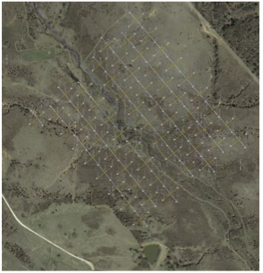
Figure 9 below shows an example layout for an existing CCUS operation, utilizing an EMgrid:
Conclusions:
spCSEM is an important new tool for the energy and mining industries with particularly beneficial applications for long-term monitoring of CCUS operations. spCSEM is especially useful in providing additional safety information by showing:
- CO2 plume lateral extent over time
- Caprock integrity
Coupled with long-term microseismic monitoring, operator’s goals for ensuring a safe and well monitored storage site can be achieved.
In addition, there are opportunities that the combined data sets provide to enhance the understanding of well integrity (the ability of wells to retain CO2 during injection, post- injection, and post-closure phases), caprock integrity, and containment risk.
References:
[1] Corwin, R. F., 1990, The self-potential method for environmental and engineering applications, in Ward, S. H., Ed., Geotechnical and environmental geophysics, 01: Soc.Expl. Geophys., 127–145.
[2] De Groot, S., 1951, Thermodynamics of irreversible processes, in J.de Boer, H., andH.B.G.Casimir, Eds., Selected Topics in Modern Physics , Vol.3: North Holland Publishing Company,Amsterdam.
[3] Ishido, T., and Pritchett, J. W., 1999, Numerical simulation of electrokinetic potentials associated with subsurface fluid flow: J. Geophys. Res., 104(B7), 15,247–15,259.
[4] Jouniaux, L., and Ishido, T., 2000, Electrokinetics in Earth Sciences: A Tutorial; InternationalJournal of Geophysics, Volume 2012, Article ID 286107, 16 pages, doi:10.1155/2012/286107
[5] Moore, J. R., and S. D. Glaser (2007), Self-potential observations during hydraulic fracturing, J.Geophys. Res., 112, B02204, doi:10.1029/2006JB004373.
[6] Revil, A., Schwaeger, H., Cathles III, L. M., and Manhardt, P. D., 1999, Streaming potential inporous media 2: Theory and application to geothermal systems: J. Geophys.Res., 104(B9), 20,033–20,048.
[7] Wurmstich, B., and Morgan, F. D., 1994, Modeling of streaming potential responses caused byoil well pumping: Geophysics, 59, 46–56.
[8] Hickey, M. S., Treviño III, S., & Everett, M. E., 2015, Monitoring and Imaging the dynamics andExtent of Hydraulic Fracturing Fluid Movement Using Ground-Based Electromagnetics, withApplication to the Eagle Ford Shale. Paper URTeC: 2172634 Presented at the UnconventionalResources Technology Conference Held in San Antonio, Texas, USA, 20-22 July 2015.https://doi.org/10.15530/urtec-2015-2172634
[9] Hickey, M. S., Treviño III, S., & Everett, M. E., 2017, Monitoring Hydraulic Fracturing FluidMovement using Ground-Based Electromagnetics, with Applications to the Anadarko Basin and theDelaware Basin / NW Shelf. Paper URTeC: 2690022 Presented at the Unconventional ResourcesTechnology Conference Held in Austin, Texas, USA, 24-26 July 2017. https://doi.org/10.15530/urtec-2017-2690022
[10] Hickey, M., Vasquez, O., Trevino, S., Oberle, J., Jones, D., & Technologies, D. I., 2019, UsingLand Controlled Source Electromagnetics to Identify the Effects of Geologic ControlsDuring a Zipper Frac Operation - A Case Study from the Anadarko Basin. Paper SPE-194313-MSPresented at SPE Hydraulic Fracturing Technology Conference and Exhibition Held in TheWoodlands, Texas, USA, 5-7 February 2019.
[11] Amanda C. Reynolds, Nabiel Eldam, Chris Galle, and Brad Bacon, Encino Energy
Trevor Pugh, Jeffrey Chen, and Suresh Dande, 2022, Subsurface Electromagnetic frac & flowback
response to natural and induced fracture networks; presentation at the SPWLA 63rd Annual
Logging Symposium held in Stavanger, Norway, June 10-15, 2022.[12] Niu, Qifei, andManika Prasad, 2016, Measurement of dielectric properties (mHz - MHz) of sedimentary rocks,SEG International Exposition and 86th Annual Meeting


