
Subsurface Electromagnetic Frac & Flowback Response to Natural and Induced Fracture Networks


Challenge
As part of ongoing efforts to optimize completion efficiency within the Utica-Point Pleasant Formation in the Appalachian Basin, surface electromagnetic arrays were set up to observe both frac water injection from the wellbore and early clean up responses. During both the initial frac and flowback, both phase and amplitude response were measured over this naturally fractured interval. The electromagnetic response of the fluids was able to determine frac geometry/asymmetry and provided ground truth to our frac modeling.
Deep Imaging® surface electromagnetic arrays were set up over the heel portion of a well. Near-wellbore natural fracture orientations and clustering were determined from both image and dipole sonic data in a horizontal well on the pad. Far-field natural fracture orientations and clustering were determined from the dipole sonic data and 3D seismic. Frac water resistivity was continuously measured from the blender. Produced water was also periodically collected and measured for its total dissolved solids (TDS).
The electromagnetic (EM) imaging provided a tool for determining the horizontal extent of the hydraulic fracture system. This allows both a check on appropriate well spacing as well as observation of the geometry of both our stimulated and drained rock volumes. This trial revealed significant stress shadowing from stage to stage in the orientation of our far-field natural fracture network.
The EM frequency response in amplitude and phase also provided a critical understanding of both the rock and areas that are successfully stimulated. We will demonstrate how anisotropic EM modeling and data show a relationship between a successfully stimulated area and the EM responses. Additionally, we will show that areas where EM flowback signal responses show the greatest change are coincident with that of the EM phase and amplitude frac signal responses.
ESG Solution
INTRODUCTION
We collected data on two adjacent wellbores from a single pad to ascertain how regional stresses and natural fractures were influencing completion and production behavior. Geomechanical and frac modeling suggested that regional stresses were likely to produce anisotropic geometries during frac’ing. Additionally, since the wellbores reside in a structurally more complex part of the acreage, we felt it necessary to also determine what effect – if any – natural fractures and more localized stresses played in the frac geometry. The longterm goal of this study is to be able to predict & optimize frac geometry once its drivers are better understood. As part of this study, EM data was collected to characterize the frac geometry, QuantaGeo® imaging and near- and far-field sonic wireline data to estimate natural fracture density, geomechnical modeling to determine the regional stresses, and perforation imaging (Dark Vision®) to estimate cluster efficiency. Additonally, 3D seismic attributes were used to determine regional representativeness of the results.
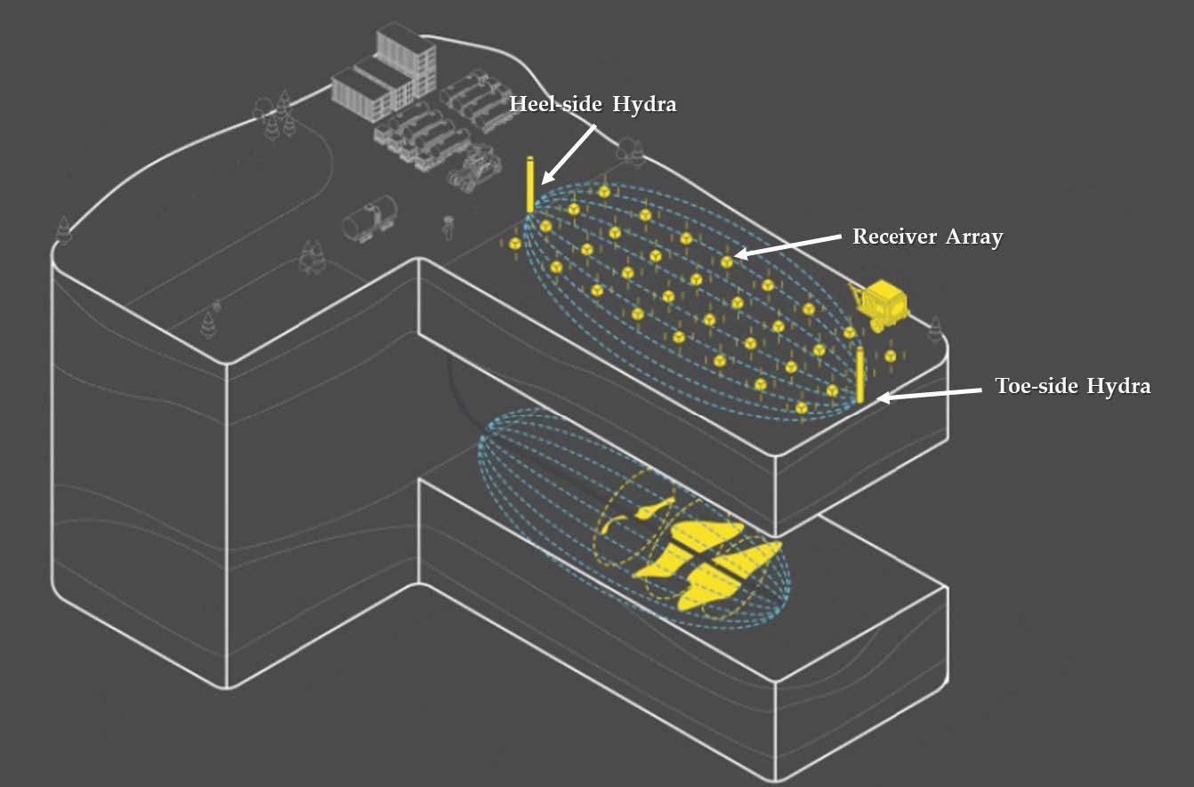
Fig. 1—Schematic of the surface EM array. Two hydras on the surface connected by a transmitter line and a receiver array on both sides designed to cover the desired lateral extent in the subsurface. Injection of conductive frac fluid perturbs the baseline EM field in the subsurface around the wellbore.
The controlled source electromagnetic (CSEM) survey (Fig. 1) was designed to capture 15 stages in the heel sections of two horizontal wells. While surface surveys do require large lead times and careful planning from a surface land standpoint, the footprint of the surface EM survey is minimal (as compared to some other geophysical survey methods) with a footprint of similar extent to that of the subsurface area of interest. Most of the monitored stages were on the westernmost well of the pad. In the neighboring well were the remaining monitored stages, the open-hole wireline data (image & triple combo), the cased-hole sonic, and the cased-hole imaging of the post-completion casing. We continuously monitored the conductivity of the frac water (a combination of both fresh and recycled water). The conductivity meter was downstream of the blender.
CSEM, commonly used in the past as a predrill verification of hydrocarbon indicators from seismic in deep water plays (Constable, 2010) has emerged in recent years in unconventional plays to track the change from earth’s baseline conductivity in response to the injection of conductive frac water. Changes in the permittivity - and, hence, capacitance – of the rock during frac’ing can be tracked with remarkable accuracy at depth. Breaking the rock causes large (104-106) changes in dielectric constant at very low frequencies (< 50Hz) in the formation (Niu and Prasad, 2016). In this paper, we will provide some results of the electromagnetic response of the formation both during frac’ing and initial flowback.
DISCUSSION
Natural fractures
The wireline image interpretation revealed several clusters of natural fractures. Their dominant orientation is NE-SW, perpendicular to the wellbore orientation and in an orientation that likely makes them critically stressed. While other natural fractures at multiple orientations were seen near-field in both the image and sonic data, sonic far-field processing revealed that only fractures in the dominant NE-SW orientation were significant in the formation. Pressure gauge data in offset wells showed the strongest pressure response to frac’ing when stages were over these natural fracture clusters. We were also able to pinpoint a seismic response to these natural fracture clusters that could be traced to the other wells on this pad and across this part of the acreage. Relevant seismic attributes also only picked up fracture clusters in the dominant orientation.
Amplitude and Phase Responses
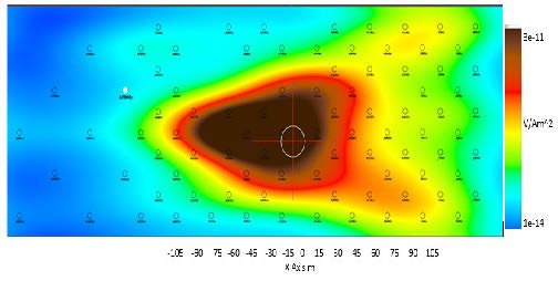
High-power extremely low frequency (ELF) Controlled Source Electromagnetic (CSEM) methods using Pseudo Random Numeric (PRN) codes have been successfully used to provide imaging of subsurface hydraulic fracturing operations. (See ref: 9-12) These techniques provide key information to better understand frac geometry. Data produced by these systems can be expressed as horizontal (aerial view) heat maps of either normalized E field in V/Am^2 or Phase in Radians. It must be noted that the discussed data is from the scatter field and not the total field. An example of a heat map response from field data can be seen in Fig. 2.
The continuous tracking of the frac water conductivity during each stage provided a necessary and critical constraint to allow the authors to interpret both the phase and amplitude spectra. Understanding the physical processes that result in amplitude and phase electromagnetic (EM) responses is vital to interpretation of the data.
There is still much debate around the best method to model the low frequency domain in 1D, 2D and 3D space. The current state of the art in 3D modeling (Haber et al., 2012) provides us a handy tool for dealing with complicated and large-scale geo-electrical models, for example, multiple long vertical and horizontal steel-cased wells, as well as multiple stage fractures, can be included in 3D EM modeling, using the efficient Octree mesh algorithm. However, to our knowledge, direct 3D simulation of anisotropic dielectric materials in the oil and gas industry has not been found in the literature yet.
Recently, several groups have started to measure electrical properties in typical formation materials under in-situ conditions. In particular, the Colorado School of Mines (Niu et al, 2016) has produced data that shows at low frequencies, dielectric constants are 5-6 orders of magnitude greater and dielectric anisotropy is 1-2 orders greater than those at frequencies > 50Hz (Fig. 3).
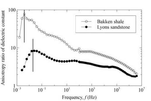
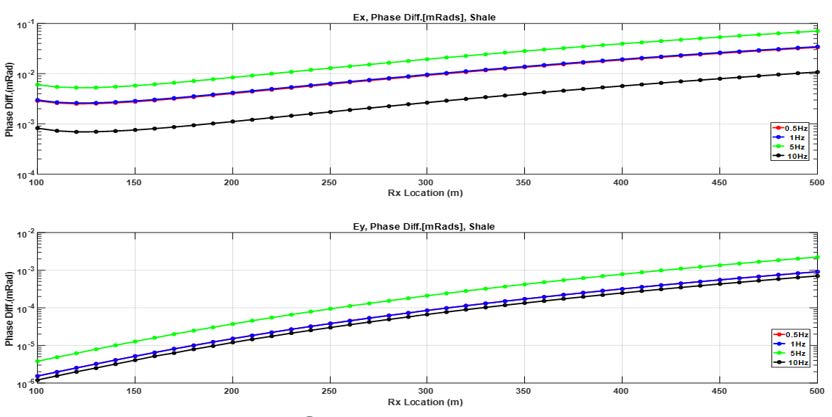
This dramatic change of permittivity can be investigated through simple 1D EM modeling, which can illustrate how changes in permittivity can affect an EM response. The modeling results show that, under the conditions modeled, there is a phase signal peak in the 5Hz region. We believe that permittivity and permittivity anisotropy are changed as a result of rock being cracked, and these changes can be seen from the EM signals in real world data, as shown in Fig.4 in a similar scenario modeling.
The measurement of frequency dependent impedance (as opposed to resistivity which is a DC measurement) is well understood in EM. There are many borehole tools using some part of the EM spectrum to produce formation impedance measurements. When frac fluid of a known conductivity is injected into a formation of known or modeled impedance and permittivity (both with anisotropic properties), we can measure changes in these properties in the EM spectrum at very low frequencies. It is required that there be a change of electrical properties only in the subsurface target structure during the period of measurement. This is so that a zero-time field (total EM field at the surface before the frac starts) can be measured and then subtracted from the EM field data collected in subsequent time steps (approximately every minute thereafter). The process is detecting changes over time in the total EM field and is very sensitive to those changes.
Amplitude and Phase of the electric fields are caused by different physical changes in the rock structure. Amplitude is affected by changes in the frequency dependent impedance (Z) and phase is affected by changes in capacitance (C) and inductance (L) in a system. The aggregate impedance of the system will change as the frac fluid is being injected into a target formation. This will result in a slowly diffusing change in the EM field at the surface. Hence, amplitude is best suited for detecting fluid transmission through the formation. The Z operator is a combination of resistance, inductance, and capacitance effects. When only amplitude changes occur (no phase shift), it can be assumed that the result is fluid movement only. The conductivity monitoring of the frac water allowed for the amplitude data to be more easily interpreted.
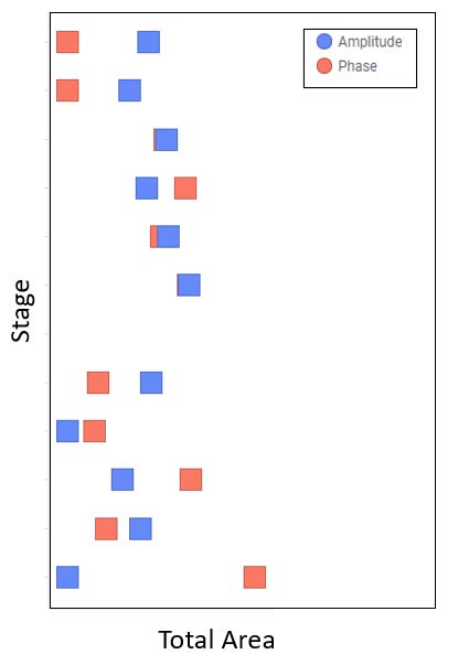
The results of this study show variability in the phase and amplitude responses seen during the frac. Figure 5 shows the total area of a signal within a stage based on both phase and amplitude responses. One can clearly see variability in both measurements and changes in which is a more dominant signal.
Since the purpose of frac’ing is to alter and to break (more complex breakages preferred) the target rock, several electrical changes can be expected from baseline in the rock. A change in anisotropic permittivity during frac’ing will lead to a phase change in EM data. In addition, with conductive fluid introduction, any polarization mechanisms due to rock layering will be destroyed. If conductive fluid is successfully introduced into the cracks created in the target rock, changes in the rocks inductive properties can also be expected. The concept depends on mutual inductance and the creation of loop circuits (Everett and Chave, 2018). This change in inductance should also be seen in the phase spectra.
Given the above, some predications can be made relating to changes in phase and amplitude spectra based on what alterations are occurring in the reservoir.
1. Amplitude only: Little or no rock cracking has occurred – maybe natural fractures, thief zone or depleted zone from adjacent parent well
2. Phase only: Rock has been broken but fluid placement is limited or over a very large area.
3. Various degrees of both responses: If amplitude response is dominant to the phase response, natural fractures may have had more influence on the frac and possibly lead to a “less complex” breakage of the rock.
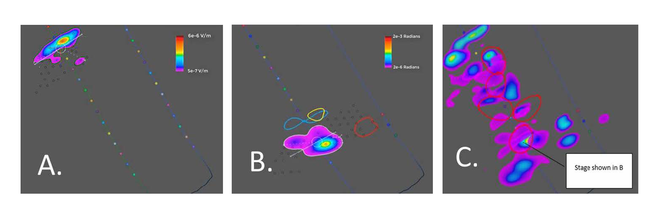
In the following examples from our data (Fig. 6), we see both phase and amplitude response variability. Examining the data in this way allows us to better understand what is driving completion behavior and likely gives hints to future stage contributions.
Figure 6a shows an amplitude-only EM response in a given stage. This stage likely corresponds to an area of higher natural fractures as determined from the image data in the offset well as well as the seismic and offset pressure responses. Perhaps not surprisingly, this stage also shows very linear growth outward in a parallel orientation to the dominant natural fractures of the area.
A different stage (Fig. 6b), on the other hand, shows a response that was approximately the same horizontal coverage area for both phase and amplitude. This is likely to have a different breakage of the rock from what was observed in Fig 6a. Note that the response on the heat map shows a much more globular shape.
Figure 6c compares the frac to a 14-day flow back EM response. There are several areas that are highlighted in red where most of the signal occurred during the flow-back period. Several observations can be made from this data when compared to the original frac data. The areas that had both phase and amplitude responses or phase and weak amplitude response are coincident with data in the flow back that has the largest response over time. The stage where only amplitude data was recorded (Fig 6a) does not show a response during flowback. The flowback data shows signal strength on alternate sides of the frac.
CONCLUSIONS
There is a clear distinction to be made when interpreting data from phase and amplitude EM measurements in frac’ing operations. It is likely that phase indicates rock being more broken up and amplitude indicates fluid is being placed. Ideally, both responses are seen. Natural fractures appear to be influencing EM response during frac. The anisotropy and “duck walking” observed in the EM data is likely a combination of regional and local stresses. Natural fracture clusters are likely to be affecting the response and most likely their orientation relative to regional stresses strengthens this affect.
There is a third signal caused by mutual inductance that can also cause phase changes. This is dependent on fractal bifurcation (Everett and Chave, 2018; Zoback and Kohl, 2019). EM modeling of this type of structure at a fine scale needs further study.
Next steps for this program include additional data collection to better understand the relationships between phase and amplitude signals and their associated completion and production responses.
For References and Authors Click HERE
Fig. 1—Schematic of the surface EM array. Two hydras on the surface connected by a transmitter line and a receiver array on both sides designed to cover the desired lateral extent in the subsurface. Injection of conductive frac fluid perturbs the baseline EM field in the subsurface around the wellbore.


